
To access the Time Scale Separation Analysis (TSSA) task in COPASI, go to the Tasks branch in the tree view on the left side of the interface and select Time Scale Separation Analysis. This will open the dialog for configuring and running the analysis.
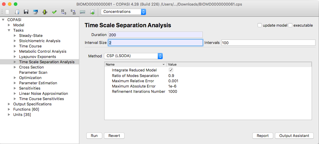 |
| TSSA Task Dialog |
The Time Scale Separation Analysis (TSSA) task in COPASI implements three methods:
These methods are designed to leverage the wide range of characteristic time scales found in biological systems. Each is based on a local analysis of the Jacobian matrix of the underlying ODEs, which is partitioned into fast and slow components at the start of an interval chosen by the user.
Depending on your chosen method, you can adjust several parameters in the Parameter value table that influence how the analysis is performed. You can find detailed explanations of each method and its parameters in the methods section of this manual. Each method provides local information at a specific time point. To gain a global picture of system behavior, you should analyze multiple time points throughout your interval of interest.
For this, you must set the Duration and either the Interval size or the number of Intervals. This is similar to performing a time course simulation. All three methods rely on numerical integration using the LSODA solver [Petzold83]. LSODA settings are set to their default values for this task and are not customizable; for details see the deterministic simulation method.
If you have not yet created a report definition, you may use the output assistant (accessible at the bottom of the TSSA task widget) to quickly set one up. You must also associate the report definition with an output file, which is done by clicking the Report button.
Once all parameters are set, you can start the calculation by clicking the Run button. COPASI will show a progress bar during the simulation, which may take longer depending on your hardware, selected method, and model size. When the calculation finishes, the Results dialog is found just below the Time Scale Separation Analysis branch in the object tree. Use the time slider in the results widget to examine results at different time points.
By default, results are displayed in the graphical user interface as tables. Positive numbers appear in varying shades of green; negative numbers are shown in shades of red. This visual coloring aids in quickly interpreting the results.
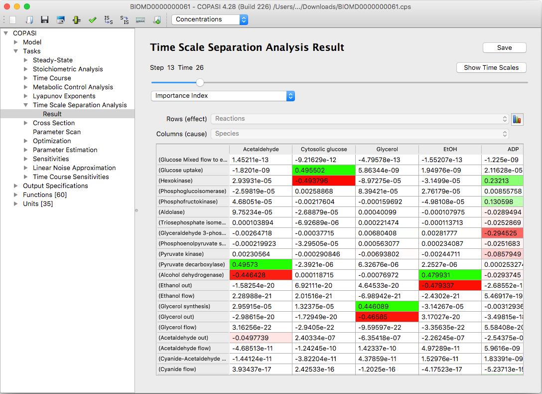 |
| An example of results table Importance Index in CSP(LSODA) method |
This makes it easy to quickly identify the most important contributions and analyze how the values are distributed. You can save these tables to a text file by clicking the Save to File button.
To visualize the results as interactive three-dimensional bar graphs, click the Bars button. COPASI uses the Qt5 Q3DBars library for these plots. You can rotate the view by holding down the right mouse button. Right-clicking also opens options for slicing the data or changing the color scheme.
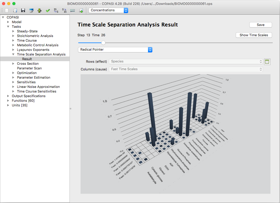 |
| An example of bar graph visualization of the Radical Pointer in CSP(LSODA) method |
The bar graphs are interactive: you can rotate and zoom them for better visibility. Additionally, you can highlight individual rows or columns in the tables to focus on specific data.
An extra diagram, available by clicking the Show Time Scales button, visualizes how the system’s time scales are distributed at a chosen time point.
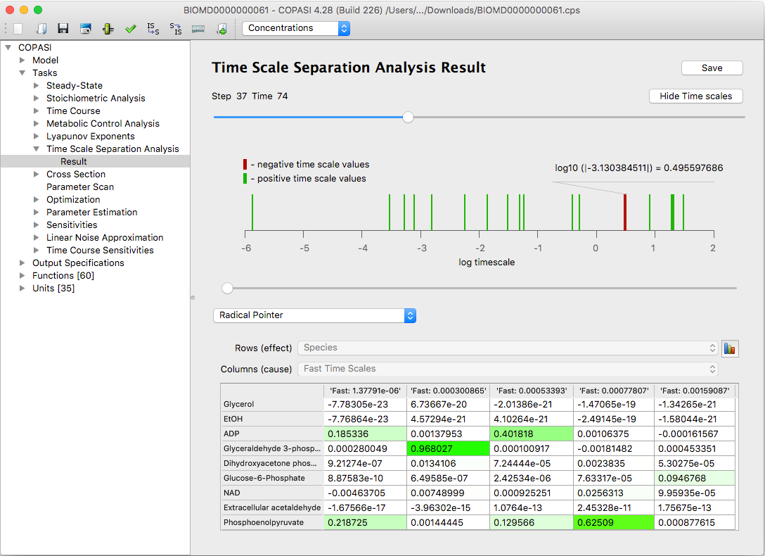 |
| An example of the time scale distribution graph |
The analysis of how time scales evolve throughout a simulation can provide valuable insights into the system’s dynamics. For more details on this approach, see Model Analysis by means of Time Scale Separation.
Fast, dissipative time scales are associated with eigenvalues of the Jacobian that have large negative real parts. Explosive modes correspond to positive eigenvalues. When time scales are equal, this typically results from pairs of complex conjugate eigenvalues, which indicate the presence of oscillatory components within the system.