
This section demonstrates how to use COPASI’s cross section task. We start by importing an oscillating model from the BioModels Database, explore its dynamics with a time course simulation, and then extract characteristic events using the cross section task.
First, download BioModel 239 from the BioModels Database. Import this model into COPASI. Then, navigate to the Tasks section, and select Time Course. Set the duration to 100 seconds and use the automatic interval size.
To visualize the simulation run, use the output assistant to create a plot for “Concentrations, Volumes, and Global Quantity Values.” Click “Hide All,” then select “[Calcium]” to show just its trace. The output will be similar to:
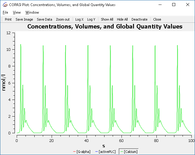 |
| Concentration time course of BioModel 239 |
To understand how changing a parameter affects the simulation, use COPASI’s
slider feature. Select Tools > Show Sliders or click the slider icon  in the toolbar. Click New Sliders and select the
“constant” parameter of reaction R2.
in the toolbar. Click New Sliders and select the
“constant” parameter of reaction R2.
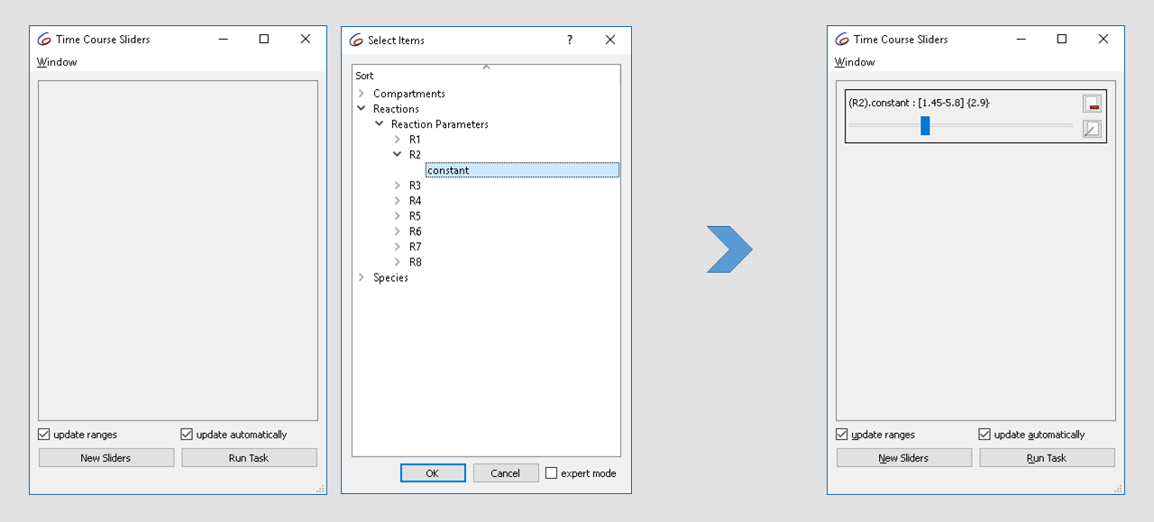 |
| Defining a slider |
The initial value is 2.9. Try changing it from 1.5 to 3 while observing the plot. You’ll see the oscillatory dynamics switch from basic oscillations to bursting:
 |
| Concentration time course while varying the slider |
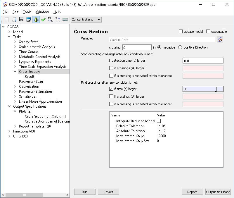
The cross section task lets you detect when the system crosses a specified value of a variable (a “surface” in phase space), in a specified direction. For this tutorial, we identify the maxima (peaks) of the previously observed calcium oscillations. Select the rate of calcium as the variable in the cross section task, detect crossings of the value zero in the negative direction, and stop detection after 100 seconds.
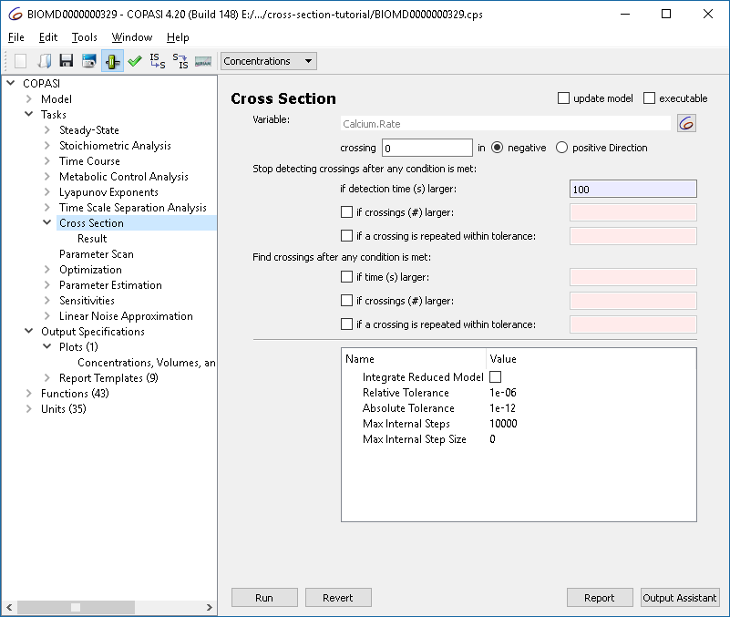 |
| Cross section task options |
To visualize results, modify the plot so that values are shown as circles rather than lines:
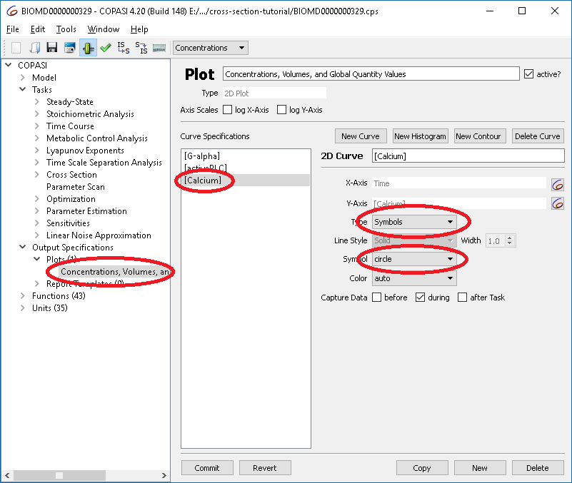 |
| Changing plot options |
Now, run the cross section task and you will obtain:
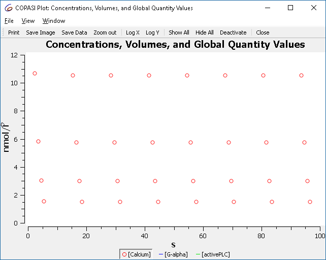 |
| Plot of cross section result, showing only maxima |
These points correspond to the maxima observed earlier.
The oscillation behavior changes when adjusting reaction R2’s parameter. We can systematically illustrate this using a scan task in combination with the cross section task to generate a bifurcation diagram.
R2.constant, varying it in 100 intervals from 1.5 to 3.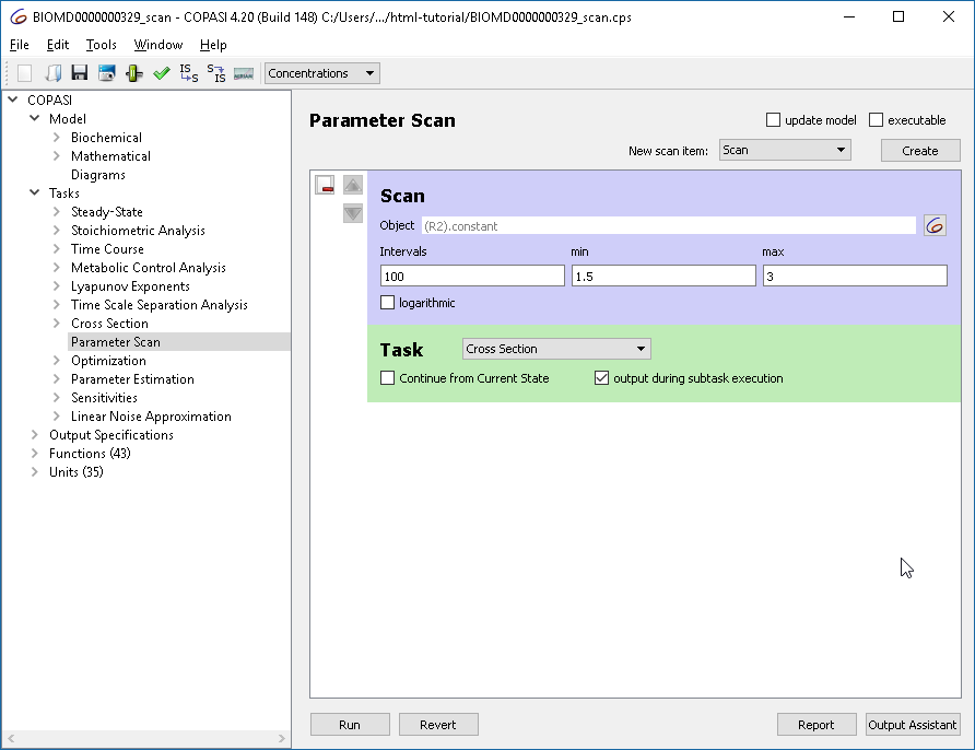 |
| Defining the parameter scan |
For the plot, set R2.constant as the x-axis and calcium concentration as the
y-axis. Use circles for points. (Alternatively, the output assistant’s “Scan of
Concentrations, Volumes and Global Quantity Values” is suitable.)
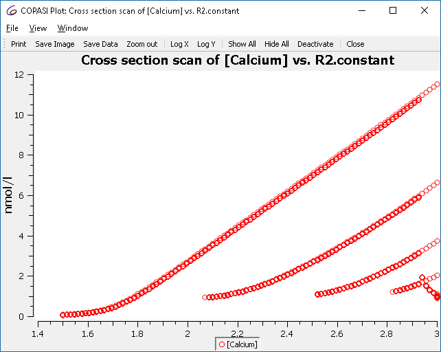 |
| Scan result: single to multiple peaks (bursting) |
This plot shows all maxima, not just those from the limit cycle. To filter for relevant crossings, configure the cross section task to only collect crossings after a certain condition, e.g., when “time > 50”.
 |
| Refining the cross section task: collect after limit cycle |
Re-running the parameter scan now yields only those crossings of interest:
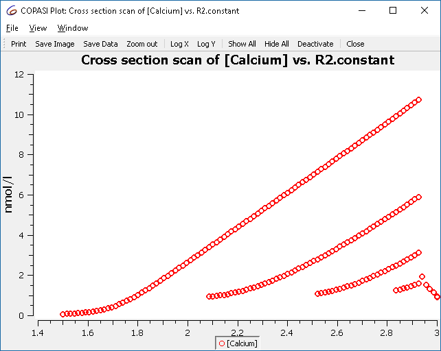 |
| Refined scan result |
The cross section task has options to efficiently find crossing points. They fall into two groups:
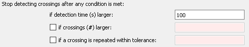 |
| Cross section termination options |
First Group: When to Stop Collecting Crossings
Note: You must set a maximum simulation time to ensure simulation ends even if crossings are absent or not repeating.
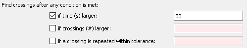 |
| Cross section collection options |
Second Group: When to Start Reporting Crossings
Complete Example Download:
Download BIOMD0000000329_scan.cps
As another example, we illustrate the route to chaos through period doubling bifurcations using a chemical-kinetics analog of Rössler’s chaotic attractor [1],[2].
As before, set up the cross section task to detect maxima of a variable (X2).
Recommended settings:
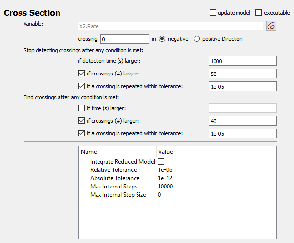 |
| Cross section options for chaotic example |
The scan task scans the autocatalytic expansion parameter from 0.05 to 0.2. Define a plot with the scan parameter on x-axis and X2 concentration on the y-axis.
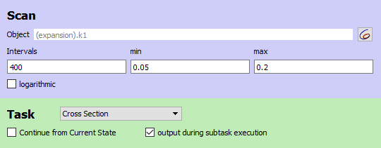 |
| Scan settings for chaotic example |
This yields the classic Feigenbaum (period doubling) diagram:
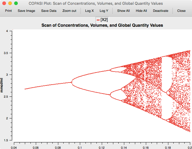 |
| Feigenbaum diagram |
Complete Example Download:
Download chaos3v2.cps
Run in COPASI
[1] O. E. Rössler: An Equation for Continuous Chaos. Physics Letters Vol. 57A no 5, pp 397-398, 1976.
[2] Baier, G., & Sahle, S. (1995). Design of hyperchaotic flows. Physical Review E, 51(4), R2712–R2714. doi:10.1103/PhysRevE.51.R2712