This page contains several examples files that allow to ascertain how a new feature in COPASI can be used to set up piecewise parameter fits that can be used for both, stochastic and deterministic models. Each example will be given as archive, that archive contains the COPASI as well as all the experimental data associated with it. To run the examples simply:
These examples have been described originally in Zimmer and Sahle (2012). They can be reproduced using the method outlined above.
For each example the archive will contain two models: the first one being the base model <file>-model.cps, it does not yet contain any events. The second model <file>-model1.cps contains the events added from zr1.txt. To select a different set of measurements we deleted events from model1.cps, replaced the experiment set of zr1.txt with the one of the other files and then regenerated the events as described above.
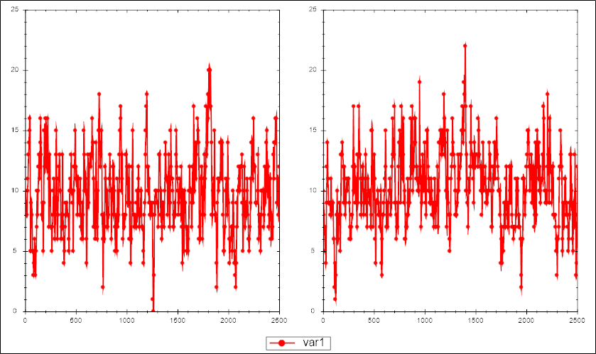
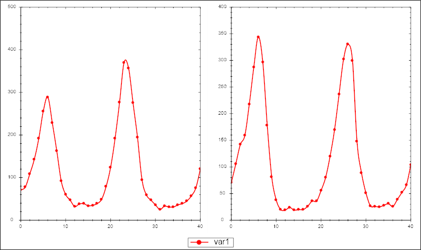
For each of the files below we give a visualization of the first to time series to give you an idea for the data
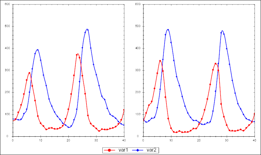
In this archive <file> will be called lv so for example lv-model.cps.
In this archive <file> will be called lvp so for example lvp-model.cps.
These examples allow to compare how the fitness landsape differs when simply applying parameter estimation (thus using a least square objective function), or using the method outlined above (thus using the MSS objective function). To compare the differences you would run the parameter estimation, once with the events being added (i.e. MSS) and then once again with the events being deleted (i.e. LSQ).
One dimensional plots of the fitness landscape can be obtained, by first finding a good fit, then changing the optimization method to Current Solution Statistic (which just evaluates the objective function), and then defining a Parameter Scan. This has already been set up in the models contained in the archives below.
This example contains four models: lv.cps,lvBIG.cps, lvmss.cps, lvmssBIG.cps. The files ending in BIG use a bigger parameter range.
This example contains four models: fhn.cps,fhnBIG.cps, fhnmss.cps, fhnmssBIG.cps. The files ending in BIG use a bigger parameter range.
This example contains seven models: calcium.cps,calciumMSS.cps, calciumMSS_2steps.cps, calciumMSS_4steps.cps, calciumMSS_10steps.cps, calciumMSS_20steps.cps, calciumMSS_50steps.cps. The different step files denote how many events have been included.